GPU-Accelerated Data Science and Machine Learning on DGX Spark
In this tutorial, you will accelerate data science and machine learning workflows on a DGX Spark using its GPU.
The Spark can be used as a standalone computer by connecting a monitor and keyboard, or as a remote server accessed from another computer. In this tutorial, we will connect to the Spark remotely and install the necessary software to run our workloads.
We will use pandas as our data processing library and scikit-learn as our machine learning library. These two libraries are foundational to the data science and machine learning ecosystem. In this tutorial, we will accelerate their workflows on the GPU using CUDA-X.
CUDA-X is the umbrella name for NVIDIA’s collection of GPU acceleration libraries. Within this collection, the set containing data science libraries is called RAPIDS. In this tutorial, we will use cuDF from the RAPIDS library suite to accelerate pandas, and cuML to accelerate scikit-learn.
This tutorial consists of three parts:
- Setup: Installing Miniconda, creating conda environments, and cloning the playbook repository
- Running the Notebooks: Running two notebooks in both CPU and GPU environments
- Comparison: Comparing CPU and GPU performance cell by cell
Setup
Connecting to the Spark
If you are connecting to the Spark remotely for the first time, you need to find its IP address. Connect a monitor and keyboard to the Spark, log in, and run the following command in the terminal:
The command outputs the IP address of the Spark’s default network interface:
Note this address; you will use it in place of throughout this tutorial. Alternatively, you can find the IP address by checking the NVIDIA Sync application.
Make sure your computer is connected to the same network as the Spark. Then, open a terminal on your computer and connect to the Spark via SSH:
On the first connection, you will see a fingerprint warning. Type yes and press Enter. Then, when prompted for a password, enter the Spark’s password:
Once connected, the Spark will start accepting commands from this terminal. Throughout this tutorial, you will enter all commands in this terminal on your computer.
Installing Miniconda
Conda is a package manager that manages Python packages and environments. If conda is not installed on the Spark, you need to install Miniconda. Run the following commands:
Verify the installation:
Add conda to your PATH:
Creating Conda Environments
In this tutorial, we will use two separate conda environments on the Spark. The first contains standard data science packages — reflecting a typical setup you may already have. Let’s call this the CPU environment. The second contains the RAPIDS libraries. Let’s call this the GPU environment.
Create the CPU environment (standard data science packages, no RAPIDS):
Create the GPU environment (includes RAPIDS libraries):
This command installs the RAPIDS 26.06 package from the rapidsai channel, CUDA 13.0 runtime from the nvidia channel, and other packages from the conda-forge channel.
After installation completes, verify the package versions:
Cloning the Playbook Repository
NVIDIA shares its DGX Spark playbooks on its website and GitHub repository . The CUDA-X Data Science playbook there contains the two notebooks we will use.
Let’s look at the directory containing the notebooks:
Two notebooks are available:
cudf_pandas_demo.ipynb— Accelerates pandas workflows with cuDFcuml_sklearn_demo.ipynb— Accelerates scikit-learn workflows with cuML
Kaggle API Key
The first notebook downloads a 4.76 GB dataset from Kaggle. To do this, you need a Kaggle API key (kaggle.json). If you don’t have a Kaggle account, sign up at kaggle.com and create an API key.
Copy the kaggle.json file from your computer to the Spark. Open a separate terminal on your computer and run the following command:
Then return to your SSH terminal and set the file permissions:
Preparing CPU Copies
To enable comparison, we will create a CPU copy of each notebook. The only difference in these copies is that the acceleration commands are commented out. All other code remains the same.
Now comment out the %load_ext line in each copy:
What Are cuDF and cuML?
In this section, before diving into the practical work, we will explain cuDF and cuML.
cuDF — pandas Acceleration
cuDF offers a “pandas accelerator mode” called cudf.pandas. This mode is activated by adding a single acceleration command to a Jupyter notebook:
When this command is run, the import pandas as pd statement loads a “proxy module” instead of the normal pandas. This proxy attempts to run every pandas operation on the GPU (via cuDF) first; if the operation is not supported on the GPU, it automatically falls back to the CPU (pandas) and synchronizes the data in the background.
Important: This mechanism requires no changes to user code. All pandas commands such as pd.read_csv(), df.merge(), and df.groupby() work as-is — they just run on the GPU.
cuML — scikit-learn Acceleration
cuML offers a “scikit-learn accelerator mode” called cuml.accel. This mode is also activated with a single acceleration command:
This command intercepts the import operations of the sklearn, umap-learn, and hdbscan modules. When you create an estimator (e.g., LinearSVC), a “proxy estimator” is created instead of the actual estimator. If cuML has a GPU implementation for that algorithm, the operation is dispatched to the GPU; otherwise, it automatically falls back to the CPU (scikit-learn).
Notebook 1: Accelerating pandas with cuDF
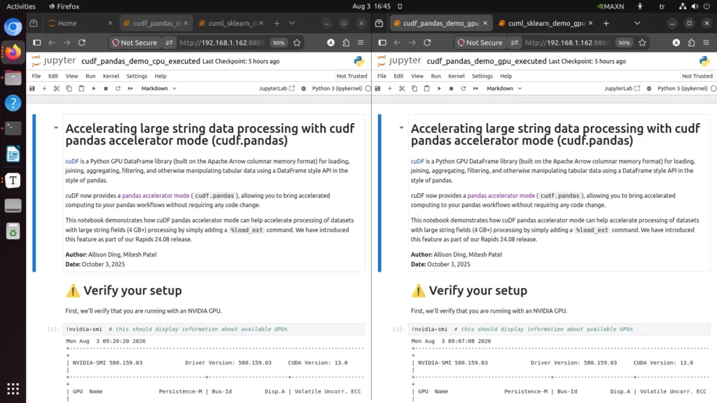
This notebook contains pandas data processing operations: loading, string operations, and grouping.
The cuDF accelerator mode (cudf.pandas) routes these operations to the GPU without requiring any code changes.
Running the Notebooks
We will run the notebooks in headless mode using jupyter nbconvert –execute. This method automatically runs all cells in the notebook and saves the outputs into the notebook file.
Running on GPU (RAPIDS environment, acceleration command active):
Running on CPU (standard environment, acceleration command disabled):
We are running the CPU copy we prepared in the “Preparing CPU Copies” section:
Notebook 2: Accelerating scikit-learn with cuML
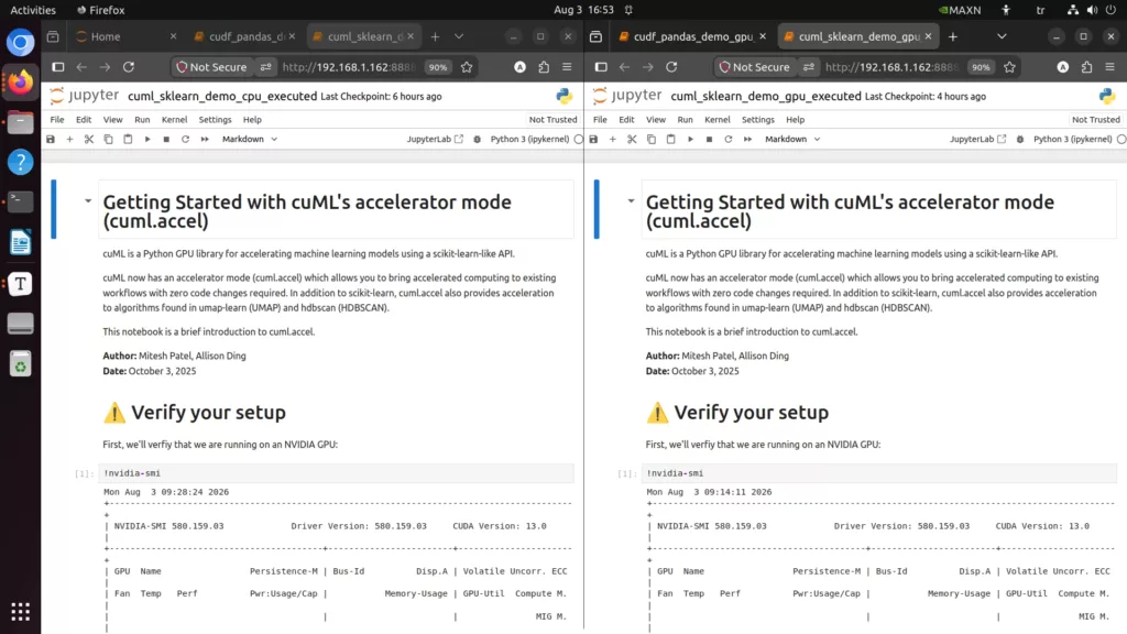
This notebook contains various machine learning operations with scikit-learn: classification, clustering, and dimensionality reduction.
The cuML accelerator mode (cuml.accel) routes these operations to the GPU without requiring any code changes.
Running
Running on GPU:
Running on CPU:
Viewing Executed Notebooks with Jupyter
Executed notebooks have all cell outputs (timings, tables, charts) embedded within them. You can view them in your browser through a Jupyter server.
Start a Jupyter server on the Spark:
Open the URL shown in the output (including the token) in your computer’s browser. In the file list on the left, you will see four executed notebooks:
cudf_pandas_demo_gpu_executed.ipynb— GPU run (cuDF)cudf_pandas_demo_cpu_executed.ipynb— CPU run (cuDF)cuml_sklearn_demo_gpu_executed.ipynb— GPU run (cuML)cuml_sklearn_demo_cpu_executed.ipynb— CPU run (cuML)
Click on any of them to view cell outputs, %%time timings, tables, and charts. You can open the CPU and GPU notebooks side by side in two browser tabs for comparison.
Comparison
In this section, we will compare important cells side by side and evaluate the results. In the screenshots, the CPU run is on the left and the GPU run is on the right.
Notebook 1: cuDF / pandas
In[4] — Acceleration Command
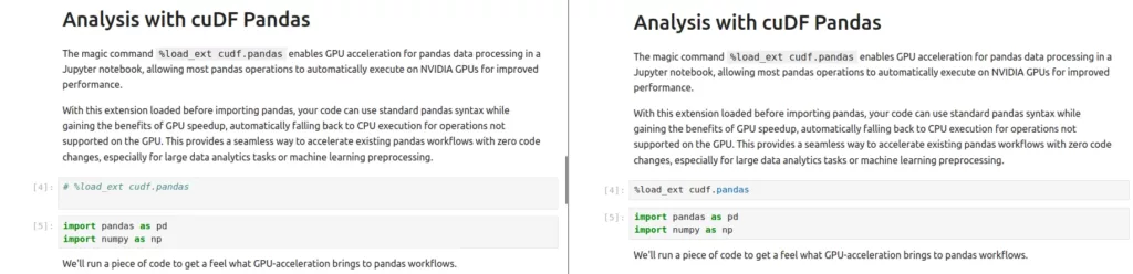
This cell is the only difference between the CPU and GPU runs. In the GPU notebook, the %load_ext cudf.pandas command replaces pandas with a proxy module. In the CPU notebook, this line is commented out (# %load_ext cudf.pandas), so normal pandas is used.
In[6] — Data Loading (4.76 GB)

Loads the 4.76 GB job_summary.csv file. This file contains the text summaries of 1.1 million LinkedIn job postings.
| CPU | GPU | Speedup |
|---|---|---|
| 25.7s | 3.87s | 6.6x |
CPU pandas reads the dataset with a single thread, which is why it is slow. cuDF’s GPU CSV reader, on the other hand, loads the data in parallel into GPU memory. For a 4.76 GB file, the time difference is very significant.
In[7-8] — Data Loading + String Operation
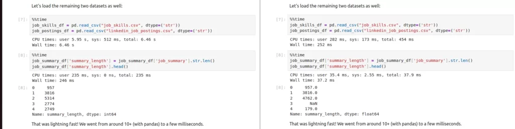
Loads two smaller CSV files (job_skills.csv 642 MB, linkedin_job_postings.csv 397 MB, totaling ~1 GB) and then calculates the length of 1.1 million strings. Calculating string length is a common operation when working with text data.
In[7] — Data loading (2 CSVs, ~1 GB):
| CPU | GPU | Speedup |
|---|---|---|
| 6.46s | 252ms | 25.6x |
In[8] — String operation (str.len() on 1.1M strings):
| CPU | GPU | Speedup |
|---|---|---|
| 246ms | 37.2ms | 6.6x |
In string operations, the GPU processes thousands of strings simultaneously rather than calculating each string’s length one by one.
In[11] — Aggregation (groupby + sort)
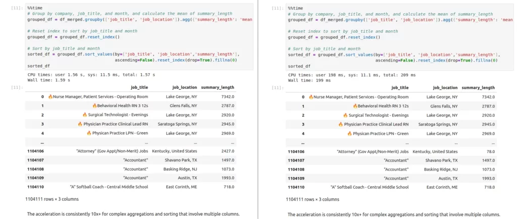
Groups 1.1 million rows by job_title and job_location columns, calculates the mean, and sorts by three columns.
| CPU | GPU | Speedup |
|---|---|---|
| 1.59s | 199ms | 8.0x |
The GPU is significantly faster in this operation.
Notebook 2: cuML / scikit-learn
In[2] — Acceleration Command

As in the previous notebook, this cell is the only difference between the CPU and GPU runs. In the GPU notebook, the %load_ext cuml.accel command intercepts scikit-learn/umap-learn/hdbscan imports.
In[7] — Classification: LinearSVC Training
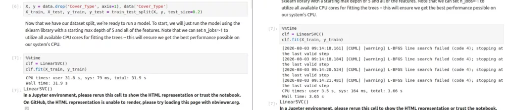
Trains a Linear Support Vector Classifier on the UCI Covertype dataset. The dataset contains 581 thousand samples and 55 features.
| CPU | GPU | Speedup |
|---|---|---|
| 31.9s | 3.65s | 8.7x |
Model training is the most time-consuming step in machine learning. The GPU performs LinearSVC’s matrix operations in parallel, significantly reducing training time. This is of great importance in scenarios where you need to train multiple models, such as hyperparameter search, which involve heavy computational workloads.
In[12] — CPU Fallback: KernelDensity
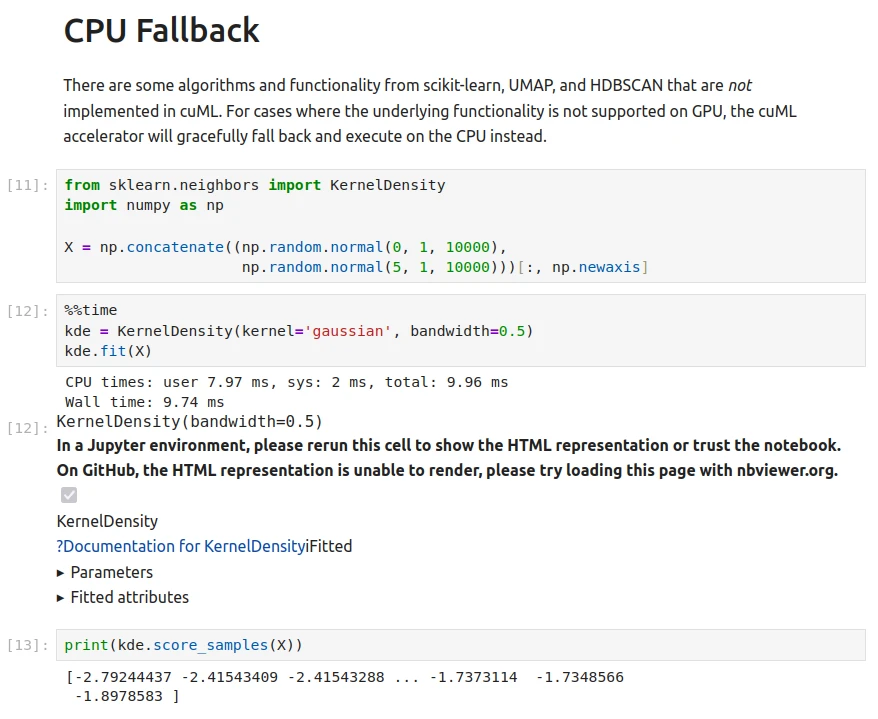
Note: This screenshot is taken from the GPU notebook only (no side-by-side comparison).
This cell is used to demonstrate cuML’s CPU fallback mechanism. The KernelDensity algorithm does not have a GPU implementation in cuML. The notebook deliberately calls this algorithm to show that unsupported operations gracefully fall back to the CPU.
| CPU | GPU | Speedup |
|---|---|---|
| 1.65ms | 9.74ms | 0.2x |
In[16] — Clustering: HDBSCAN
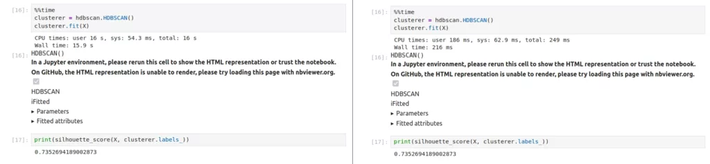
HDBSCAN is a density-based clustering algorithm. Here it runs on synthetic data (20 thousand samples, 100 features, 5 clusters).
| CPU | GPU | Speedup |
|---|---|---|
| 15.9s | 216ms | 73.6x |
This is the largest speedup recorded during this tutorial. HDBSCAN involves computationally intensive steps such as density calculations and minimum spanning tree construction. These steps can be accelerated dozens of times by leveraging the GPU’s parallel processing power.
In[25] — Dimensionality Reduction: UMAP

UMAP reduces high-dimensional data to a lower dimension (here, 561D → 2D). The UCI HAR dataset (7,352 samples, 561 features) contains human activities recorded from smartphone sensors.
| CPU | GPU | Speedup |
|---|---|---|
| 13.9s | 367ms | 37.9x |
UMAP involves building a k-NN graph and various optimization steps. These steps provide significant parallelization advantages on the GPU.
Conclusion
In this tutorial, we accelerated pandas and scikit-learn workflows on the DGX Spark using CUDA-X libraries (cuDF, cuML) on the GPU. We ran two notebooks in both CPU and GPU environments to make a real performance comparison.
The results obtained:
| Operation Category | Typical Speedup |
|---|---|
| CSV loading | 6-25x |
| String operations | 6x |
| groupby + sort | 8x |
| LinearSVC training | 8.7x |
| HDBSCAN clustering | 73.6x |
| UMAP dimensionality reduction | 37.9x |
The most striking results were achieved with the HDBSCAN (73.6x) and UMAP (37.9x) algorithms. This is because these algorithms involve intensive mathematical computations, which is where the GPU’s parallel processing power provides a significant advantage.
These results show that by adding a single command to your pandas and scikit-learn code running on the Spark, you can achieve significant speedups. We also recommend trying these notebooks on your own computer. This is because whether GPU acceleration is present or not, the performance of the DGX Spark’s 20-core ARM CPU may surprise you!
Shutdown
When you are done, stop the Jupyter server with Ctrl+C. The conda environments you created on the Spark (cpu-baseline and rapids-test), the executed notebooks, and the downloaded datasets remain on disk — nothing is deleted.
To view the notebooks again, restart the Jupyter server:
When the server starts, open the URL containing the token shown in the terminal in your browser.